| The Problem: |
| In many cars the engine or the circuit of cooling water are cooled by forced convection. In fact, it is easily observable that the engine temperature goes down when the car is moving: air with a given velocity cools better the engine than air still with respect to the engine. How can we verify the effect of moving air in a process of cooling? |
| Learning aims: |
|
• Make students aware of different aspects of convection in air. • Make students aware of how experimental evidence can help them to decide on an everyday problem. • Gain abilities in collaborative work aimed at design and carry out an experimental investigation. • Gain abilities in reflecting on the purpose and nature of experimental activities they carried out in the unit. |
| Materials: |
|
• Two squares of aluminium (side ≅ 15 cm, depth ≅ 3mm), • Two temperature surface sensors • A bowl with hot water ( about 90°C) • Two plastic bags • Two isolating supports (Styrofoam) |
| Suggestions for use: |
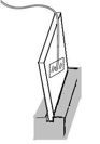  |
| Figure 3_2a) Figure 3_2b) |
|
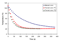
Two squares of aluminium (side ≅ 15 cm, depth ≅ 3mm), previously heated at a temperature of about 90°C (for details see Classroom activities ) are set on Styrofoam isolating blocs (see figs 3.2a) and 3.2b) ) and are leaved cooling by air at room temperature. Fig. 3.2a) shows the case of natural cooling and Fig. 3.2b) the case of forced cooling. Temperature are registered by two surface sensors previously posed in contact with one square surface using two pieces of scotch.
Figure 3_2c) |
| Possible questions: |
|
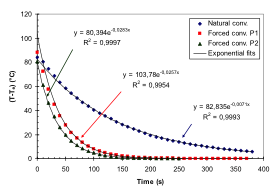
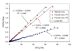
1. Compare the three curves shown in figure 3_2c and say what are the main differences? 2. What are the main differences between the two curves representing forced convection? NOTE em> An analytical expression for the cooling curves can be obtain through fitting procedures (Figure 3_2d) or by representing data in a different format. Figure 3_2e) give an example of data fitting obtained by plotting the opposite of the temperature to time difference ratios ( – ΔT/Δt ) as a function of the temperature increase with respect to the environmental (T-Te) (see Classroom materials).
|